Abstract. This research paper analyzes the relationship between the share of value added in the service sectors of the Azerbaijani economy in GDP (Y) and the volume of investments made in tourism-related sectors (X1), the number of foreigners and stateless persons accommodated in hotels and hotel-type establishments (X2), and the number of overnight stays by foreigners and stateless persons in hotels and hotel-type establishments (X3). Using the Eviews8 application software package, a regression model was constructed, graphical representations were analyzed, the correlation coefficient and descriptive statistics were calculated, and stationarity was investigated using the Dickey-Fuller test. Additionally, the presence of autocorrelation between the levels of time series was examined. The existence of heteroskedasticity in the constructed model was investigated using the White test.

Keywords: econometric model, regression equation, F-Fisher criterion, T-Student criterion, correlation coefficient, heteroskedasticity, stationarity, Dickey-Fuller test.      

                                                          Main Results of the Research

Statistical data for the econometric research were obtained from the official sources of the State Statistics Committee of Azerbaijan. Annual statistical indicators from 2009 to 2022 were used in this study. To construct a multivariate linear regression model and ensure the effectiveness of the results, the natural logarithms of the mentioned indicators were applied. The dynamic representation and descriptive statistics of the logarithmic time series are shown in Graph 1 and Table 1:

Graph 1.

                                             Graphical Represantaion of Dynamic data

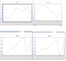
Table 1

Descriptive Statistics of Variables (Based on Logarithms)

Here, positive skewness values indicate right-skewed asymmetry, while negative skewness values indicate left-skewed asymmetry. The high kurtosis values observed indicate that the data has more extreme values than a normal distribution.

The econometric model is generally expressed by the following regression equation:

                 lnY=α_0+α_1 lnx_1+α_2 lnx_2+α_3 lnx_3+lnε_t,

Where:

Y is the share of value added in the service sectors of the economy in GDP (percentage),

x_1- is the volume of investments made in tourism-related sectors (in million manats),

            x_2- is the number of foreigners and stateless persons accommodated in hotels and hotel-type establishments (number of people),

            x_3- is the number of overnight stays by foreigners and stateless persons in hotels and hotel-type establishments (number of nights).

The Least Squares Method was used to estimate the parameters of the analyzed model. The regression coefficient indicates how much the dependent variable changes (in its measurement unit) when an independent variable increases (or decreases) by one unit in its measurement unit. Using the Eviews8 software package, the parameters of the linear regression models estimated by the Least Squares Method are described in Table 2.

Table 2.

Multivariate Linear Regression Model

The multivariate function obtained through the Least Squares Method allows us to determine which variable has a stronger impact on the dependent variable. By using this function, it is possible to show the relationship between the logarithmic indicators of the variables in the model. The formal description of the constructed regression model is as follows:

                     LNY = 0.00717226488627*LNX1 + 0.574472518735*LNX2 –

                             - 0.595346588679*LNX3  +4.00405970007

Based on Table 2, let us evaluate the significance of the constructed model. The value of the coefficient of determination (R2=0.635586R^2 = 0.635586R2=0.635586) indicates that approximately 64% of the variance in the dependent variable is explained by the model. The aggregate correlation coefficient shows the degree of closeness between the dependent variable and the explanatory variables included in the model. The closer this indicator is to 1, the stronger the relationship between the outcome factor and the set of factors. In this case, the relationship is quite strong.

To verify the significance of the constructed model, we apply the F-Fisher test. To check the significance of the regression equation using the theoretical econometric method, the calculated F-statistic value is compared with the table value of F (at the chosen significance level of 5%). The model is considered significant if the calculated F-statistic is greater than the corresponding critical value of the F-Fisher statistic, i.e., Fcalculated>FtableF_{calculated} > F_{table}Fcalculated>Ftable.

Using the Eviews8 software package, the significance of the model was analyzed with the F-Fisher criterion. The Prob. value of the F-statistic test, which characterizes the significance of the model, was 0.014507. Since Prob F-stat = 0.014507 < 0.05, the model can be considered significant.

In general, evaluating the significance of the regression equation involves determining whether the mathematical model describing the relationship between variables fits the experimental data and whether the number of explanatory variables included in the equation is sufficient to describe the dependent variable.

The significance of the parameters was tested based on the T-Student criterion. To theoretically check the significance of the model using the T-Student criterion, the inequality ∣tcalculated∣>ttable|t_{calculated}| > t_{table}∣tcalculated∣>ttable is tested. The T-Student statistical test, which characterizes the significance of the parameters, was checked using the Eviews software package. For each parameter to be considered significant individually, the inequality Prob T statistic < 0.05 must be satisfied. According to the observed values, the parameters X2X_2X2 and X3X_3X3 are considered significant. Based on the results in Table 2, although the significance condition is met for other parameters, the parameter X1X_1X1 cannot be considered significant as Prob T statistic = 0.8392 > 0.05 based on the T-Student criterion.

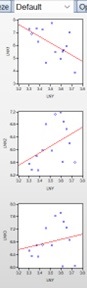
The graphical representation of the regression line of the constructed model is shown in Graph 3.

Graph 3.

Graphical Representation of the Regression Line

The significance of regression models can also be analyzed through correlation analysis. In correlation analysis, measuring and evaluating the strength of the relationship between the variables in the regression model is crucial. Since the constructed econometric model is multifactorial, multivariate correlation analysis was conducted. To determine the correlation dependence, the values of the correlation coefficient are examined, and based on the obtained results, the strength of the correlation is identified as strong, moderate, or weak. The correlation coefficient can take values from negative one (-1) to positive one (+1):

A correlation coefficient close to -1 indicates a strong negative linear relationship between the variables. A value close to +1 indicates a strong positive linear relationship, while a value close to zero indicates the absence of a linear relationship. Based on the indicators of the correlation matrix, the strength of the relationship between the factors is evaluated using the Chaddock scale.

According to this scale, if the value of the correlation coefficient is less than 0.3, the dependence is weak; between 0.3 and 0.7, the dependence is moderate; and greater than 0.7, the dependence is strong. The results of the correlation analysis are described in Table 3. According to Table 3, the correlation coefficient between LN_X2 and LN_X3 (r=0.954117) is close to one, indicating a perfect positive correlation between these factors. This suggests the presence of multicollinearity between the factors.

Table 3.

Correlation Matrix of Factors

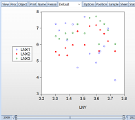
The correlation plot for the factors is depicted in Graph 4. This graph illustrates the relationship and the strength of correlation between the variables included in the regression model. By examining this plot, one can observe how the variables interact with each other and identify any strong linear relationships or patterns.

Graph 4.

Correlation Plot for Factors

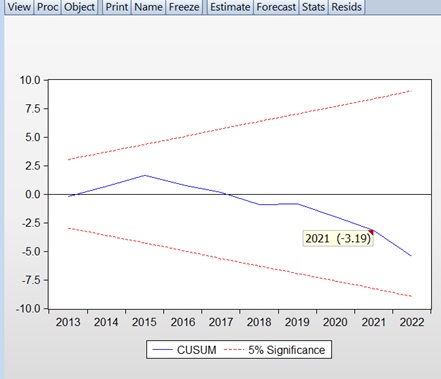
The assessment of the stability of a regression model is crucial in terms of its adequacy and structural analysis. The stability of the model can be examined using the CUSUM test. This test is also employed in econometric and statistical research to detect unexpected changes in the parameters of regression models over time. The CUSUM test is based on the calculation of the cumulative sums of recursive residuals and the cumulative sums of the squares of the recursive residuals, as well as the evaluation of the corresponding equations. The test results are represented by diagrams showing the dynamic changes of these values, with 95% confidence intervals established for them. If the recursive estimates of the residuals exceed the critical boundaries, it indicates parameter instability in the model. Given that the CUSUM chart is cumulative, even minor shifts in the process will result in a continuous increase (or decrease) in cumulative deviation values. Therefore, detecting trends and shifts in the process through the CUSUM test allows for timely adjustments.

Using the Eviews8 software package, the stability of the parameters for the constructed multivariate regression model was tested with the CUSUM test. The results of the CUSUM test are shown in Graph 5. In Graph 5, the blue line remaining within the red lines indicates the acceptance of the null hypothesis H0H_0H0 of parameter stability, meaning that our model is considered stable.**

Graph 5.

 CUSUM test

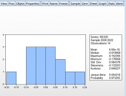
Checking the fulfillment of the Gauss-Markov conditions for the residuals of an econometric model is crucial for assessing its adequacy. In Graph 6, using the Eviews8 software package, the fulfillment of the Gauss-Markov conditions for the residuals of the model has been examined. This description includes the Jarque-Bera statistic, which indicates the normality of the distribution. Additionally, this statistic serves as an indicator for checking whether the residuals meet the Gauss-Markov condition of normal distribution. According to the Eviews8 software package, if the Probability value of the Jarque-Bera statistic is greater than 0.05, the residuals are considered to follow a normal distribution with 95% confidence. Otherwise, the residuals do not follow a normal distribution. Based on Graph 6, since the Probability = 0.973255 > 0.05, the hypothesis that the residuals follow a normal distribution is accepted.

Graph 6.

Checking Gauss-Markov Conditions for Residuals 

To evaluate the adequacy of the regression model, the approximation error is used. Suppose that for each value of the parameter xxx, two different values of the parameter yyy are compared: the actual yyy and the estimated value from the regression model. The Mean Absolute Percent Error (MAPE) expresses the deviation of the mean value of the computed y^hat{y}y^ from the actual  y^hat{y}y^​  as a percentage:

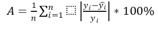
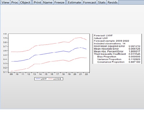
Using the EViews software package, the significance of the regression model can be assessed by the Mean Absolute Percent Error (MAPE). If the MAPE value is less than 5-7%, it indicates that the given information has been processed well based on the model. Otherwise, the model might be considered unsatisfactory. According to the results shown in Graph 7, our model has a Mean Absolute Percent Error (MAPE) of 1.86% < 6%, suggesting that the model is adequate.**

Graph 7.

Investigating heteroskedasticity and homoskedasticity is crucial in econometric modeling. The term heteroskedasticity is used when the covariance matrix of the error vector is diagonal but with varying diagonal elements. In other words, errors from different observations are not dependent on each other, but their variances differ.

The fulfillment of this initial condition is called homoskedasticity (the stability of the dispersion of residuals). Failure to meet this condition is termed heteroskedasticity (the instability of the dispersion of residuals).

Using the EViews8 software package, heteroskedasticity can be assessed graphically and through various tests.

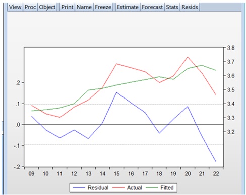
Graphically, heteroskedasticity can be checked using the residual plot. For this purpose, the Actual, Fitted, and Residual Graphs are analyzed. Visual inspection of the Residual Graph allows for the identification of heteroskedasticity. In Graph 8, the Residual Graph shows that deviations (dispersions) are sometimes very large and sometimes small, indicating heteroskedasticity in the residuals.

Graph 8.

Actual Fitted Residual Graph 

The heteroskedasticity of the studied model has been examined using the White test, with results presented in Table 4. This test was conducted using the EViews8 software package

Table 4.

Results of the White Test for Heteroskedasticity

If the p-value of the determination coefficient is greater than 0.05, the null hypothesis of homoskedasticity is accepted. This indicates that, as per the Gauss-Markov condition, the residuals exhibit constant dispersion and there is no heteroskedasticity. Conversely, if the p-value is less than 0.05, heteroskedasticity is present in the model.

The Dickey-Fuller test is widely used to check for the stationarity of time series data. This test is applied to verify the unit root hypothesis in time series data. If the p-value of the Dickey-Fuller test is less than 0.05, the null hypothesis of a unit root is rejected, and the alternative hypothesis of stationarity is accepted. Additionally, the value of the Dickey-Fuller test must be smaller than the critical values at the 1%, 5%, and 10% significance levels to confirm stationarity.

Now, let us analyze the stationarity of the variables in our regression model using the results of the Dickey-Fuller test from the EViews 8 software package. According to the results in Table 5, we can assess the stationarity of the time series. Based on our test results, all variables are non-stationary at the initial level and at first differences. However, they become stationary at second differences, with no presence of a trend or unit root.

Table 5.

Results of the Dickey-Fuller Test

A correlogram can be used for the diagnostics of time series data. Using the EViews 8 software package, the correlogram of the constructed model is presented in Figure 9.

Figure 9.

Correlogram of the Time Series

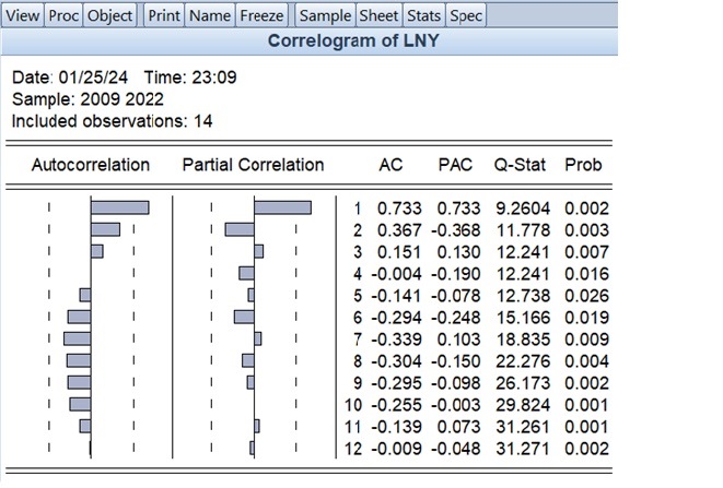
The graph in the Autocorrelation (AC) and Partial Correlation (PAC) columns shows the graphical representation of the selected autocorrelation and partial autocorrelation functions.

Additionally, the corresponding confidence intervals are also visible in the table (indicated by dashed lines). The numerical values of the selected autocorrelation and partial autocorrelation functions for different lags are shown in the AC and PAC columns (lags are listed in the third column).

In the Q-Stat and Prob columns, the Ljung-Box Q-statistic value and the p-value for this statistic are provided. The Ljung-Box Q-statistic tests the null hypothesis of no autocorrelation for up to the k-th order or less (i.e., autocorrelation coefficients are equal). The k-th order Ljung-Box Q-statistic is calculated using the following formula:

            Q=T(T+2) ∑_(k=1)^m▒(r_k^2)/(T-k)

            T = number of observations

            Rk= k-th order autocorrelation

            m = number of lags tested

Since the p-value is greater than zero and less than 0.05, the null hypothesis of no autocorrelation among the levels of the time series cannot be rejected at a 99% confidence level, indicating the presence of autocorrelation.

Additionally, the Durbin-Watson statistic can be used to detect autocorrelation between levels of time series. For the multivariate regression models we constructed, the presence of autocorrelation between the levels of the time series was examined using the Durbin-Watson criterion.

To accomplish this, we first determined the critical bounds for the Durbin-Watson statistic based on the number of observations in the model (14 observations). According to the critical bounds table for the Durbin-Watson statistic, the segment [0.4] was divided into five parts, with the bounds set as dL=1.05d_L = 1.05dL=1.05 and dU=1.35d_U = 1.35dU=1.35.

Table 6 shows that the observed value for the Durbin-Watson statistic is dobs=1.004d_{obs} = 1.004dobs=1.004. Since 0<dobs=1.004

Table 6.

Mechanism for Testing the Durbin-Watson Statistic 

Conclusion

The analysis conducted reveals that modern econometric methods can be effectively applied to the study of processes occurring within the Azerbaijani economy. The macroecono-mic indicators used in this research cover annual data from 2009 to 2022. The econometric model was  constructed and analyzed using the EViews8 software package. Based on the results from the multivariate regression model analysis, it is evident that both investments and the influx of tourists have an impact on the GDP.

Unfortunately, despite Azerbaijan's diverse tourism potential, it has not yet fully transformed into a major tourism hub in the region. To meet the high demands of incoming tourists, it is necessary to conduct further research in the tourism sector and leverage the experiences of developed countries. Considering the strong competition in the tourism sector, entrepreneurs must ensure the continuous development and renewal of their services. This will enable them to align their offerings with the ever-increasing demands of tourists.

Econometric analysis has identified a strong dependency between the volume of investments in tourism-specific sectors and the number of tourists arriving in the country. To remain competitive in the coming years, special attention should be given to investments in hotels and restaurants.

REFERENCES

1. Johansen, S. Statistical Analysis of Cointegration Vector //Journal of Economic Dynamics and Control, 1988, 12, p. 231—254.

2. Johansen, S., Juselius, K. Maximum Likelihood Estimation and Inference on Cointegration with Applications to the Demand for Money //Oxford Bulletin of Economics and Statistics, 1990, 52, p. 169—210.

 3. Granger, C.W. Investigation Causal Relations Econometrics Models and Cross-Spectral Methods //Econometrica, 1969, 37, p. 424—439.

4. https://www.stat.gov.az/

5.Stepen J. Page. Tourism Managment: An Introduction. 4-th edition Published bu Elsener. 2001

6.Technical Assistance for the Development of Tourism Strategy in Azerbaijan. Caspian Consulting Baku, 2006